From Flash Attention to Speculative Decoding: The Most Comprehensive Guide to LLM Inference Acceleration

About 2040 wordsAbout 7 min

2026-07-01

Anyone who has used ChatGPT knows that the model takes seconds or even tens of seconds to generate a response. Where is the bottleneck? Is there a way to make large language models "speak faster"? This article starts from the underlying principles and breaks down 6 major categories of acceleration techniques to help you build a complete inference acceleration knowledge framework.

01 A Core Question: Why Is LLM Generation So Slow?

To understand acceleration methods, you first need to understand how large language models actually generate content.

The process of text generation in an LLM is essentially a word-by-word completion game:

The model first reads your input Prompt (this is called the Prefill phase, processing all input tokens at once)
Then it generates one word at a time (this is called the Decode phase, generating one token at a time)

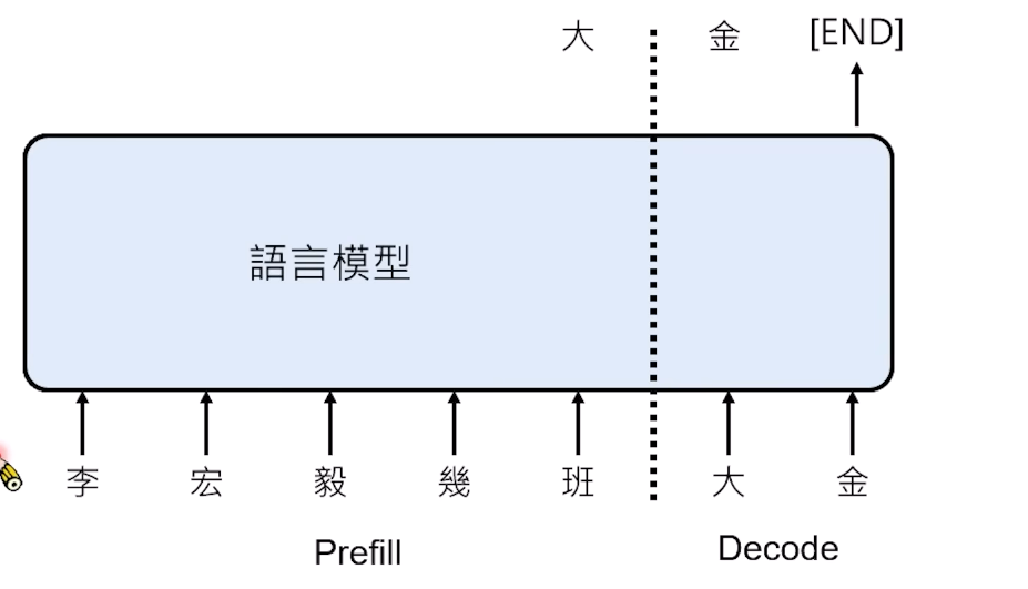
So how does each step actually compute? This brings us to the core module of the Transformer — Self-Attention.

In simple terms, each token generates three vectors: Query, Key, Value. When generating the next token, its Query computes a "similarity score" (dot product) with the Keys of all previous tokens, then uses this score to weight and aggregate all Values.

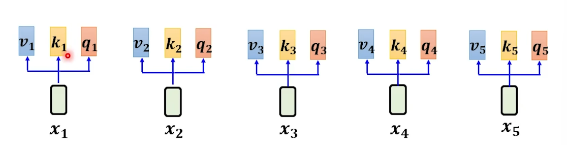
See, here's the problem:

Every time you generate a token, you have to compute attention with all preceding tokens.
The more tokens there are, the more computation is required, and the longer the wait.

So how do we accelerate this? Academia and industry have developed a series of methods, and they can be used in combination. Let's break them down one by one.

02 Flash Attention: Changing the Algorithm Doesn't Change the Formula, Only the Data Movement

Paper: https://arxiv.org/abs/2205.14135

In One Sentence

Flash Attention doesn't change the attention computation formula — it changes the order of computation to reduce data movement, thereby achieving significant speedup.

Understanding GPU Architecture

To understand why Flash Attention is fast, you first need to know how GPUs work:

GPUs have many Execution Units that perform arithmetic
Each execution unit has a small "workbench" — SRAM, extremely fast but very small
Bulk data is stored in a "warehouse" — HBM (High Bandwidth Memory), large capacity but slow to read/write

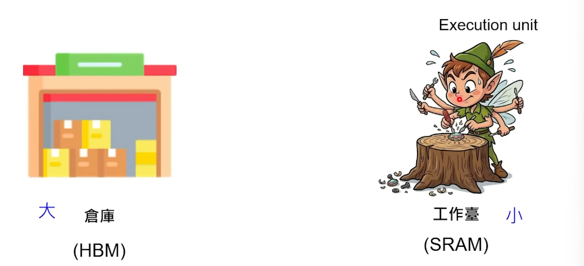
So for each operation, the execution unit must first move data from HBM to SRAM, compute, then move it back.

The bottleneck of Attention computation isn't slow computation — it's slow data movement.

Traditional Attention computation takes several steps, each requiring HBM read/write:

Move Q, K → compute dot product → move result back to HBM
Find maximum → move back to HBM
Compute denominator (Softmax sum) → move back to HBM
Compute final attention weight → move back to HBM
Move V in for weighted sum → move result back to HBM

Throughout the process, HBM is repeatedly read and written.

The Core Idea of Flash Attention

Flash Attention merges all these steps — it doesn't need to compute the full attention weight before doing weighted sum. It computes and merges on SRAM in one go.

Specifically, it splits K and V into multiple chunks and processes one chunk at a time. The key trick is:

When processing the next chunk, if you find the previous chunk's max value was too small, you can adjust the previously computed results with a correction term without recomputing.

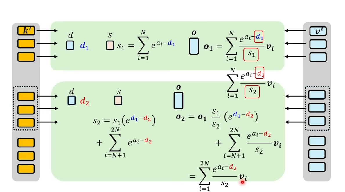
Expressed as a formula:

When processing the 2nd chunk, the previously computed $o_1$ needs adjustment:

o_2 = o_1 \frac{s_1}{s_2}(e^{d_1 - d_2}) + \sum^{2N}_{i=N+1}{\frac{e^{a_i - d_2}}{s_2}v_i}

This formula looks complex, but the core idea is simple: Multiply the previously computed part by a "correction factor" — no need to recompute.

Effectiveness and Limitations

✅ No change in results: Mathematically equivalent to standard Attention
✅ Plug and play: Can be directly used on any model with Attention
✅ Significant speedup: The longer the sequence, the more obvious the effect
⚠️ If the sequence is too short, the speedup is less noticeable

03 KV Cache: Trading Storage for Speed

Core Idea

In the Decode phase, every time a token is generated, the model must compute attention with all previous tokens. But previous tokens don't change, so their K and V don't need to be recomputed.

KV Cache stores the K and V of previous tokens, computing only the new token's QKV each time, avoiding redundant computation.

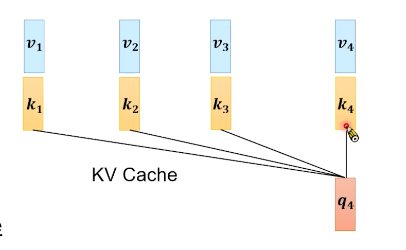
This idea is simple and direct, and it doesn't change the Attention computation logic at all.

The Cost: Memory Explosion

The problem with KV Cache is obvious — it consumes too much memory.

Every time a new token is added, a new set of K and V must be stored. And it's not just one set — Transformers have multiple layers × multiple heads of K and V.

Let's calculate with Gemma 2:

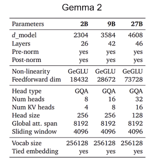
\text{Per Token: } 46(\text{layers}) \times 32 (\text{heads}) \times 128 (\text{dim}) \times 2 (\text{FP16}) \times 2(\text{V, K}) = 753664 \text{ bytes} (\text{about 736KB})

Note that this is for one token. If the sequence length is 114k, the A100's 80GB VRAM is completely filled.

KV Cache makes the model faster, but it eats up a lot of VRAM, limiting the context length that can be processed.

This is the core contradiction of the KV Cache acceleration approach.

04 Reducing KV Storage: Three Ways to Make the Cache More Efficient

Since KV Cache takes up too much space, can we store less K and V? Here are three classic approaches:

Approach 1: Multi-Query Attention (MQA)

In Multi-Head Attention (MHA), each head has its own K and V. MQA's idea is:

Multiple Query heads share a single set of K and V.

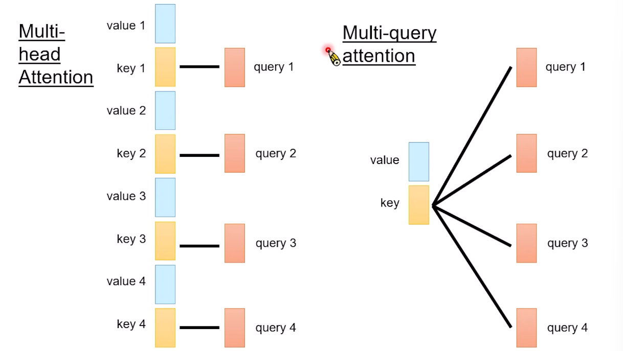
The benefit is a large reduction in KV Cache, but the problem is also clear: sharing one set of K/V is too aggressive, and model performance degrades.

Approach 2: Grouped-Query Attention (GQA)

GQA is a compromise: divide Query heads into groups, with each group sharing one set of K and V.

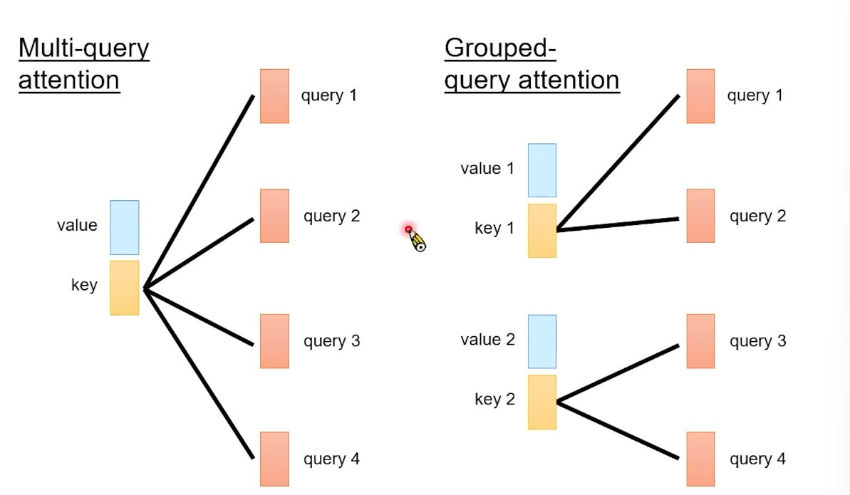
It sits between MHA and MQA, balancing efficiency and effectiveness. Many new models (like Llama 2/3) use GQA.

Approach 3: Multi-head Latent Attention (MLA)

Paper: https://arxiv.org/abs/2405.04434 (DeepSeek)

MLA's idea is more ingenious: instead of storing K and V directly, compress them into a low-dimensional vector first, and don't necessarily need to decompress when using them.

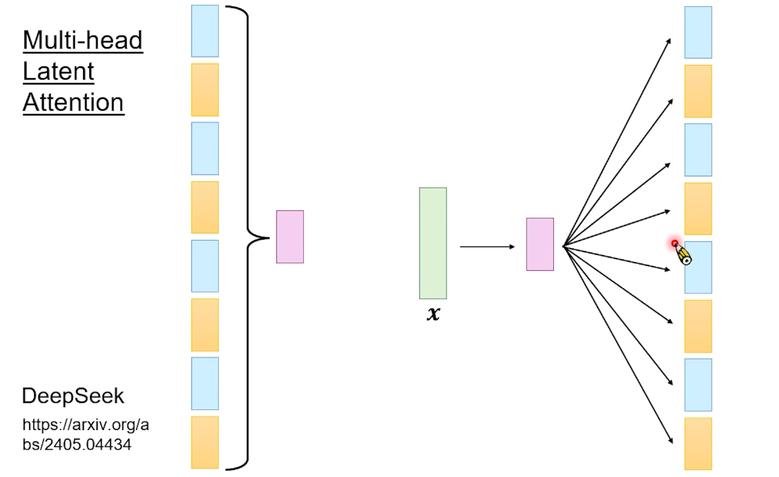
This involves two key techniques:

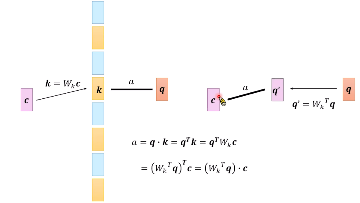
Technique 1: Dot product in compressed space

Compress input X into vector $c$ , and store this $c$ . When computing Attention:

a = q \cdot k = q^T k = q^T W_k c = (W_k^T q)^T c = (W_k^T q) \cdot c

See, you don't need to decompress $c$ into $k$ — just transform $q$ and do dot product in the compressed space.

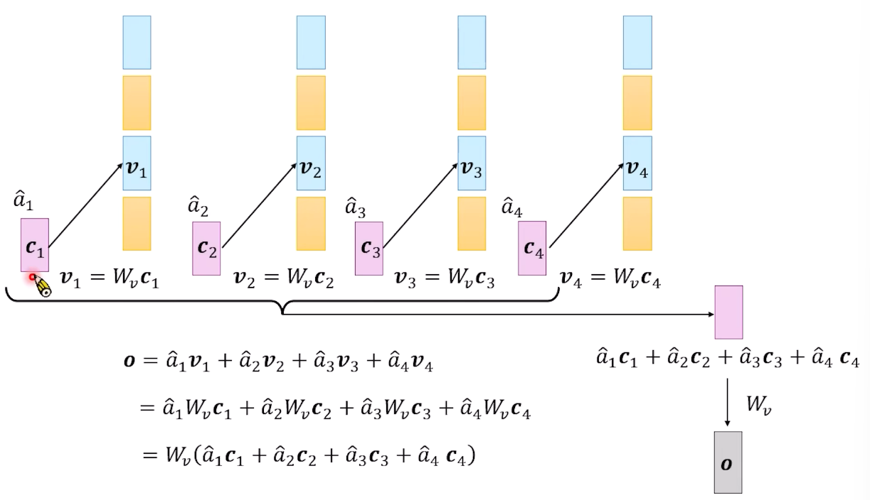
Technique 2: Weighted sum in compressed space

After computing attention weights, do weighted sum to get the output:

\begin{align*} o &= \hat{a}_1 v_1 + \hat{a}_2 v_2 + \hat{a}_3 v_3 + \hat{a}_4 v_4 \\ &= \hat{a}_1 W_v c_1 + \hat{a}_2 W_v c_2 + \hat{a}_3 W_v c_3 + \hat{a}_4 W_v c_4 \\ &= W_v (\hat{a}_1 c_1 + \hat{a}_2 c_2 + \hat{a}_3 c_3 + \hat{a}_4 c_4) \end{align*}

Key insight: Do weighted sum on the compressed $c$ first, then decompress only once at the end. This greatly reduces computation.

MLA requires retraining the model, but its adoption by cutting-edge models like DeepSeek proves this path is viable.

05 Sliding Window Attention + Streaming LLM: Only Looking at Nearby Content

Sliding Window Attention

The core idea is simple: When computing Attention, don't look at the entire sequence — only look at the nearest N tokens.

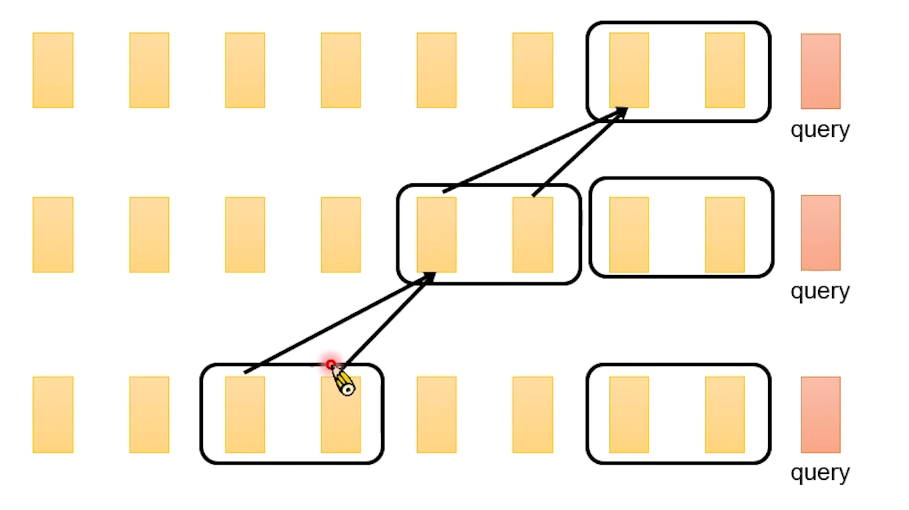
But won't the model lose long-distance information? There's a clever observation:

The deeper the Transformer layers, the larger the effective receptive field of Sliding Window Attention.

Because layer 1 only looks at nearby tokens, but layer 2's input already contains the information from layer 1's window, effectively expanding the receptive field. If the network is deep enough, even small windows can cover long ranges.

Hybrid Strategy

Another approach: Some layers use Sliding Window, others use global Attention.

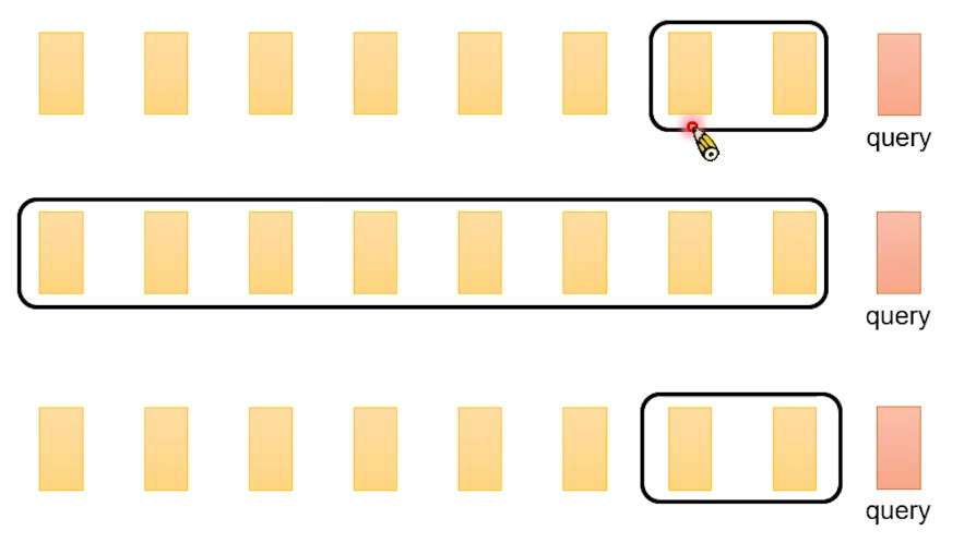
This saves KV Cache while maintaining global视野 in key layers.

Streaming LLM

Paper: https://arxiv.org/abs/2309.17453

There's an interesting finding: Using only Sliding Window degrades performance, but if you keep the first few tokens, it works well.

And this approach doesn't require retraining — just modify the inference code.

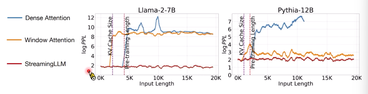
Experimental results show that Streaming LLM significantly outperforms pure Window Attention on long sequences.

06 Pruning KV Cache: Discarding Unused K and V

Here's a more direct approach: If some K and V are never used, why not just discard them?

Research has found that Attention is actually very sparse — most tokens have very small attention weights, almost unused.

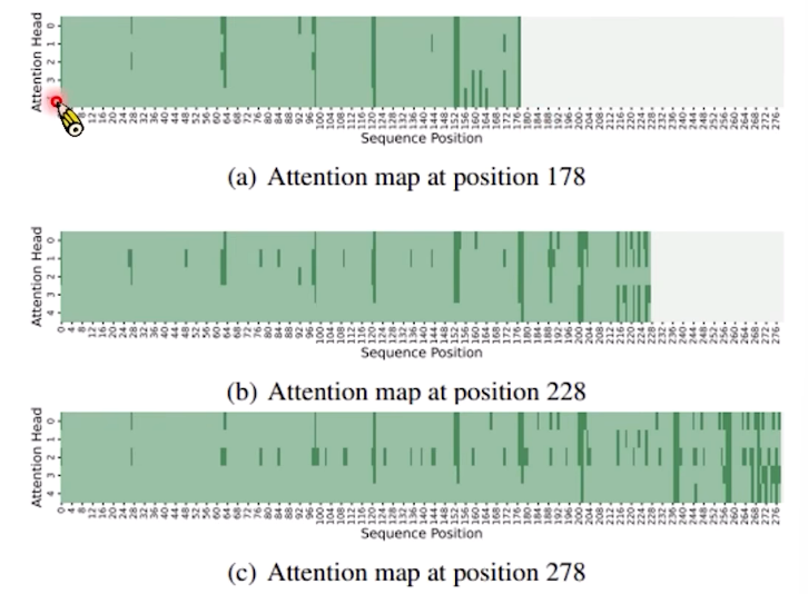
Darker colors indicate larger attention weights. As you can see, only a few tokens are actually attended to.

Based on this observation, two papers proposed different pruning strategies:

Scissorhands (https://arxiv.org/abs/2305.17118)
H2O (https://arxiv.org/abs/2306.14048)

The core idea is the same: If a K/V hasn't been used by Attention for a long time, remove it from the Cache.

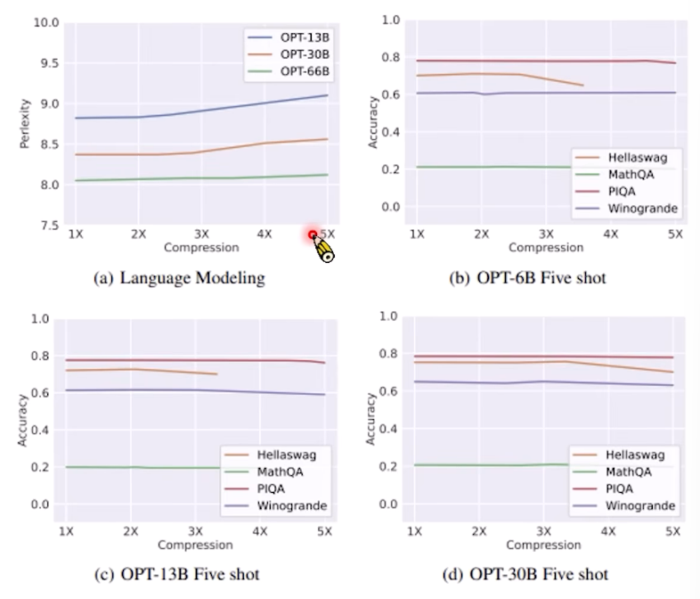
Scissorhands experiments show that with 5× compression, model performance is essentially the same as without compression.

But ⚠️ subsequent research also found: when models are given very difficult tasks, arbitrarily discarding K/V can cause significant performance degradation. This method is suitable for routine tasks but should be used cautiously in critical scenarios.

07 Cross-Conversation Cache: A Game Changer for Agent Scenarios

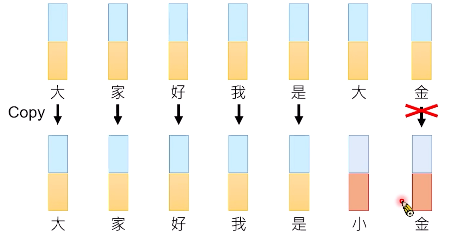
The KV Cache approaches discussed so far are all optimizations within the same conversation. But KV Cache has an even more advanced application — sharing across conversations.

If the same text segment appears in different conversations, their K and V can theoretically be reused.

Which Scenario Benefits Most?

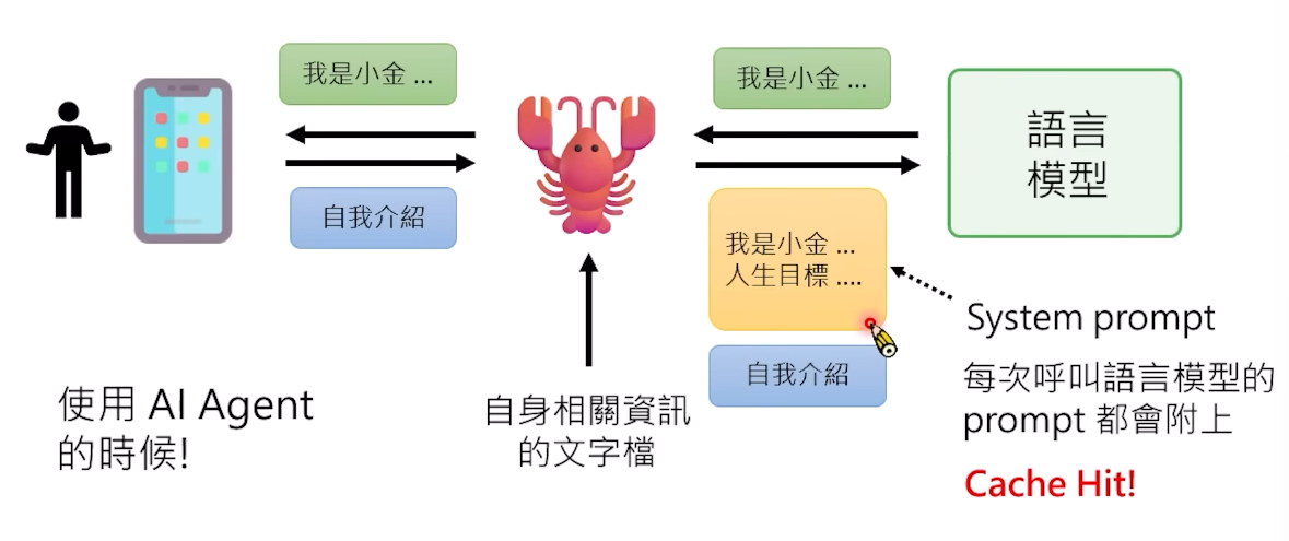
AI Agent scenarios are the perfect stage for cross-conversation Cache:

Every Agent call carries a System Prompt (role settings, tool definitions, memory instructions, etc.), and these contents are highly consistent across different conversations.

Usage Tips

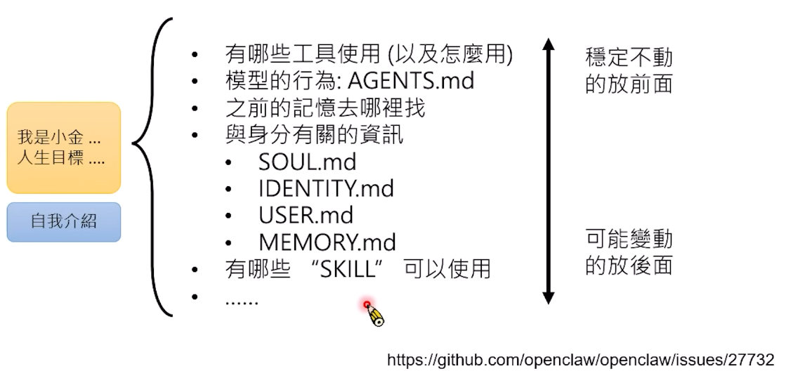
To maximize Cache Hit rate, the order of content matters:

Place more stable, unchanging content earlier, and more variable content later.

Additionally, different phrasings of the same Prompt can yield vastly different Cache Hit rates:

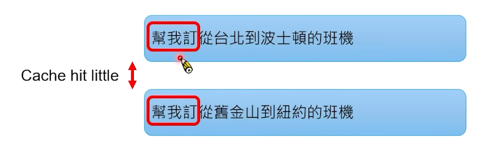
After rewriting, Cache Hit significantly improves, which means direct cost savings.

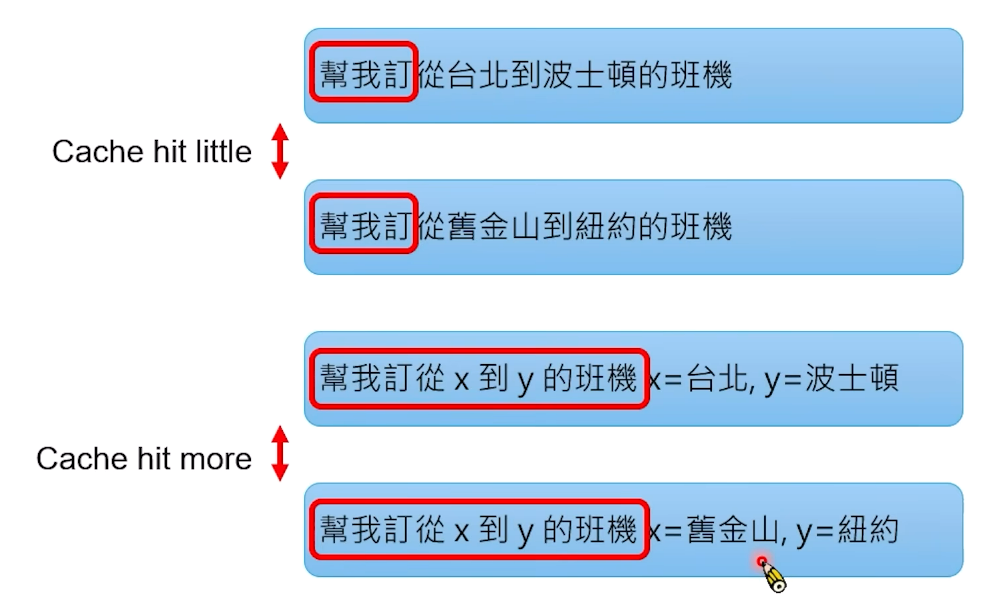
A paper specifically measured this effect: https://arxiv.org/abs/2601.06007

The conclusion: With good Prompt writing combined with Cached Input, Agent costs can be substantially reduced.

08 Summary: All Acceleration Methods at a Glance

Method	Description	Changes Attention?	Needs Training?	Main Cost
Flash Attention	Reduce HBM reads/writes, optimize compute order	✗	✗	Some extra computation
KV Cache	Store computed K and V, avoid recomputation	✗	✗	Large VRAM usage
Multi-Query Attention	Multiple Query heads share one K/V set	✓	✓	May hurt model capability
Grouped-Query Attention	Query groups share K/V	✓	✓	Efficiency-quality balance
Multi-head Latent Attention	Compress K/V before storing	✓	✓	Needs retraining
Sliding Window Attention	Attend to nearby tokens only	✓	?	May lose long-distance info
Streaming LLM	Sliding Window + keep initial tokens	✗	✗	—
Pruning KV Cache	Discard infrequently used K and V	✓	✗	May degrade on hard tasks
Speculative Decoding	Small model drafts, large model verifies	✗ (theoretically)	✗	Extra computation for small model

References

Flash Attention: https://arxiv.org/abs/2205.14135
Multi-head Latent Attention (DeepSeek): https://arxiv.org/abs/2405.04434
Streaming LLM: https://arxiv.org/abs/2309.17453
Scissorhands: https://arxiv.org/abs/2305.17118
H2O (Heavy-Hitter Oracle): https://arxiv.org/abs/2306.14048
Cached Input impact on Agent costs: https://arxiv.org/abs/2601.06007

Copyright

License under:Attribution 4.0 International (CC-BY-4.0)