
The Most Complete Breakdown of LLM Positional Encoding: Absolute, Relative, Rotary, and No Positional Encoding at All
Abstract: Transformer's Self-Attention itself does not perceive token order — shuffling the tokens of "the cat ate the fish" produces exactly the same Attention output. This article systematically traces the complete technical evolution of Positional Embedding: from the clock-hand analogy of Sinusoidal absolute positional encoding, to ALiBi and T5 relative positional biases, to the mathematical principles of RoPE (Rotary Position Embedding), and finally exploring Train Short Test Long extension methods and the "no positional encoding" NoPE/DroPE approaches.
Copyright Ownership: Kstheme, Contributors: Kstheme
01 A Basic Question: How Does Transformer Know the Order of Tokens?
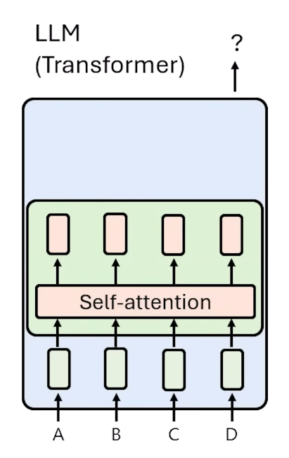
The original Transformer has no way to consider the order of input. How does it process input tokens?
Input tokens become Embeddings, which then become inputs to a Layer. Each layer contains Self-Attention, which outputs another set of tokens.
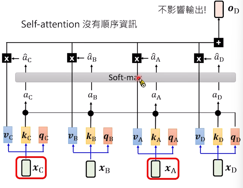
But there's a problem: Self-Attention itself does not consider the order of input tokens.
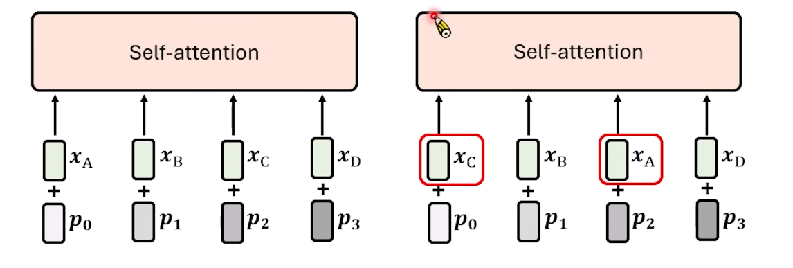
If I swap the positions of Token A and Token C and compute Self-Attention again, you'll find that the output is completely unaffected.
So we must find a way to "inject" positional information into the Transformer. This is what Positional Embedding solves.
This article covers:
- Absolute Positional Embedding (Sinusoidal)
- Relative Positional Embedding (ALiBi, T5)
- RoPE (Rotary Position Embedding)
- Train Short, Test Long (Position Interpolation, Frequency-Based Methods, YaRN, Dynamic Scaling, LongRoPE)
- No Positional Embedding (NoPE, DroPE)
02 Absolute Positional Embedding
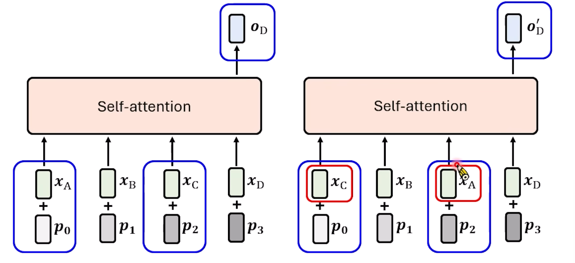
The earliest Positional Embedding idea was straightforward: assign a special Embedding to each position. This Embedding represents positional information.
We use through to represent the special Embedding for each position, then add this Embedding to our vectors.
When tokens change order, their Embeddings become different, and the final Self-Attention output also differs.
Sinusoidal Positional Embedding
Reference: https://arxiv.org/abs/1706.03762
This Positional Embedding existed from the birth of the Transformer.
Let represent the length of the Embedding ().
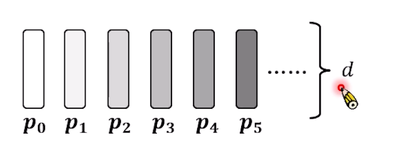
We use to represent its values.
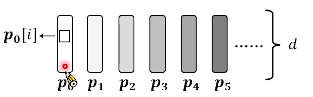
How does Sinusoidal Position Embedding construct all Embeddings? The formula is:
Visual Understanding
If we take through , we'll see a Sine function.
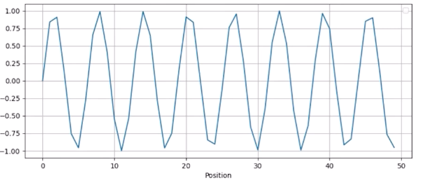
Next, through form a Cosine function.
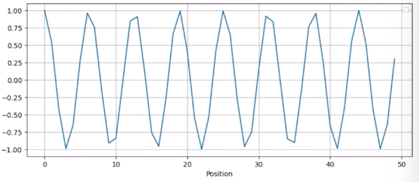
Next, through also form a Sine function, but with a larger period.
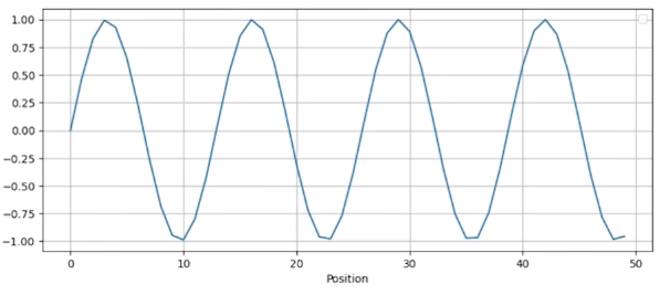
Plotting all Position Embeddings would look like this:
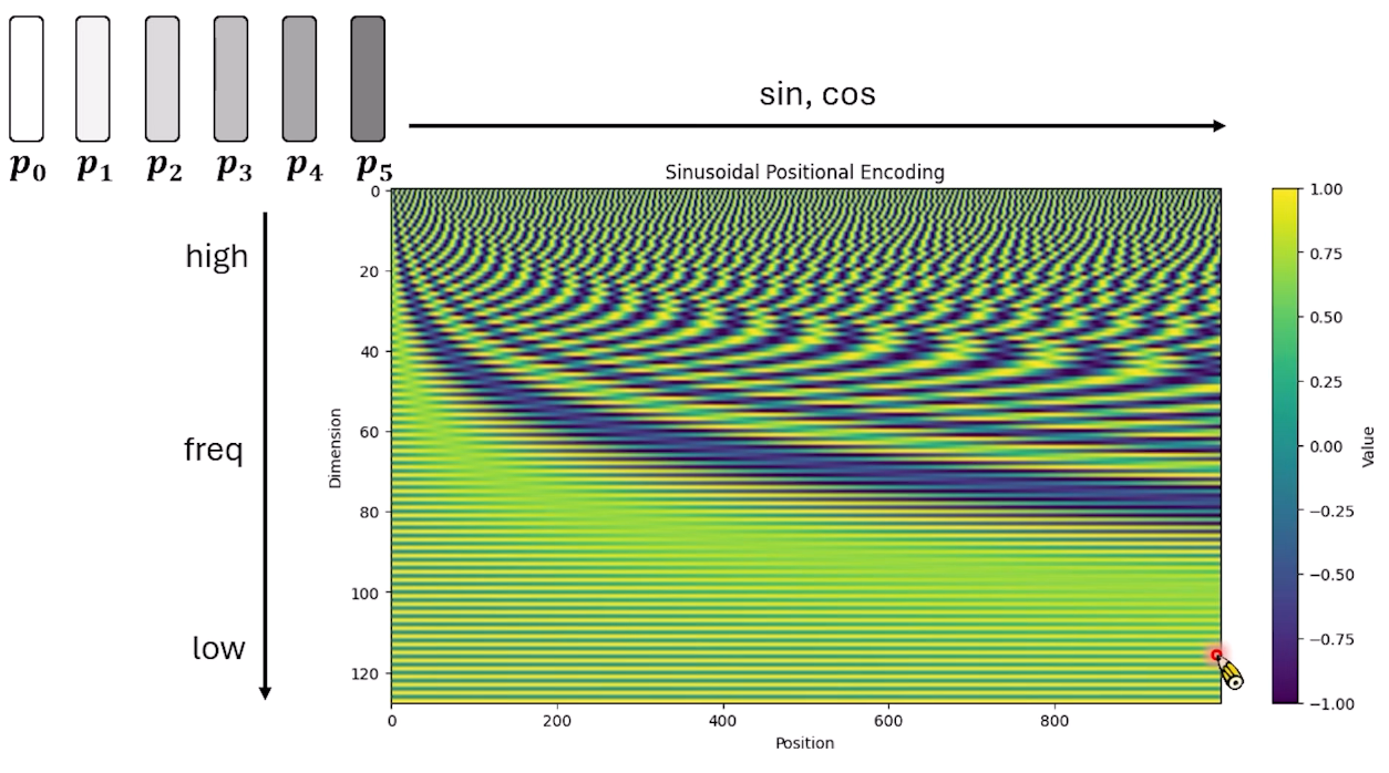
Clock Hand Analogy: Second Hand, Minute Hand, Hour Hand
We can view Sinusoidal Positional Embedding differently: even dimensions use Sine, odd dimensions use Cosine. So we can imagine each pair and as a 2D vector (a clock hand on a 2D plane). This hand rotates as increases — when rises, the hand rotates counterclockwise.
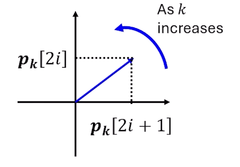
The rotation period is:
The number of needed for one full rotation:
If , then .
Different values have different periods:
| value | value |
|---|---|
| (dimensions 0, 1) | 6.3 |
| (dimensions 64, 65) | 628.3 |
| (dimensions 126, 127) | 54410.1 |
The first two dimensions rotate fastest — about 6.3 tokens per cycle. Dimensions 10-11 rotate more slowly. Dimensions 100-101 barely change within the first 6 tokens.
Every two dimensions form a hand. The fastest is the second hand, slower is the minute hand, slowest is the hour hand. With dimension 128, we have 64 hands. The Transformer uses these 64 hands and their positions to determine each token's location.
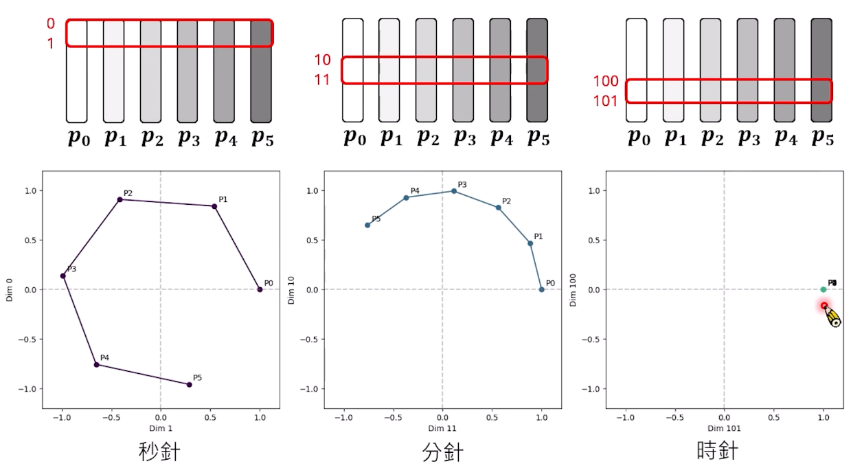
Using clock hands to represent position seems reasonable, but why did the authors choose this approach? Because they wanted Positional Embedding to handle Relative Position.
Relative Positioning is Crucial!
Relative Position means: in the sentence "the cat ate the fish," cat and fish are two tokens apart. When Transformer considers which token should follow fish, it looks back at cat. Fish's attention score for cat is 0.7.
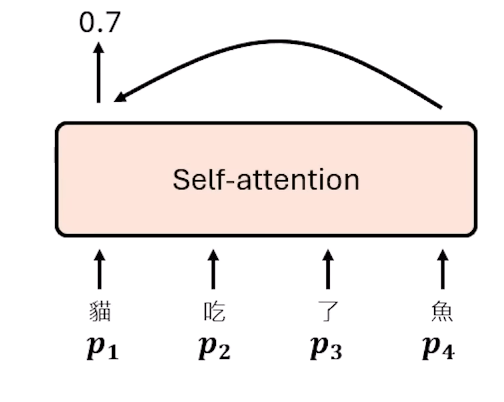
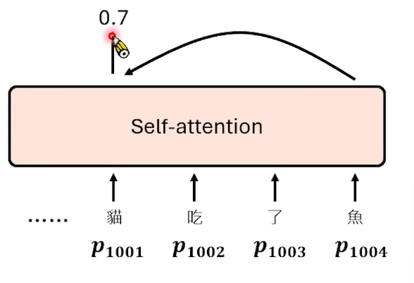
If I insert many tokens before cat — say 1000 tokens — but the relative position between cat and fish remains unchanged, we want fish's attention on cat to remain unchanged. Even if fish is at position 1004 and cat at 1001, fish's attention score for cat remains 0.7.
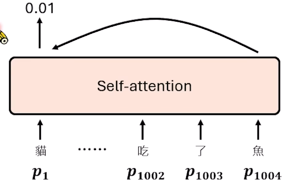
But if cat is at position 1 and fish at position 1004 — very far apart — we want fish's attention score for cat to be small.
Sinusoidal Positional Embedding was chosen because it has special properties that help with Relative Position.
Where represents position and represents position .
This formula is independent of — it only depends on the relative position between and :
Let's examine how Sinusoidal Positional Embedding satisfies the Relative Position condition.
Position formula:
Position formula:
Using sine and cosine addition formulas:
Expand :
In matrix form:
The rotation matrix is denoted as .
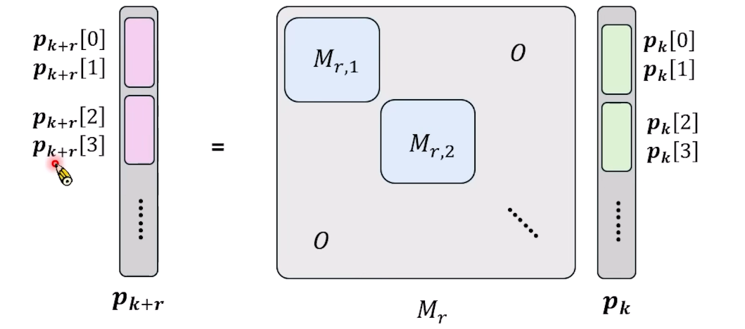
How does this design affect Self-Attention? Using and for positions, the attention score is:
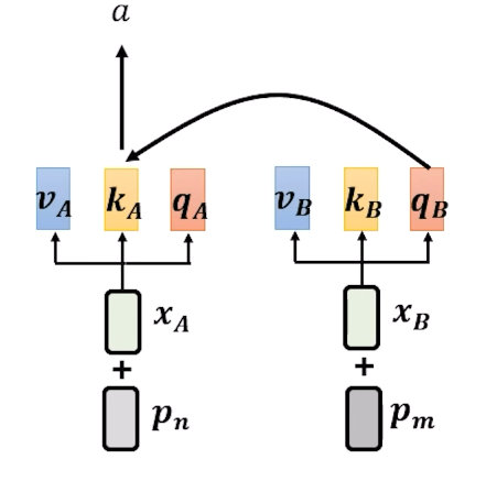
The term shows absolute position. Converting to relative position:
Where only depends on the relative position, but the overall formula still contains absolute position correlations.
03 Relative Positional Embedding
Since using Absolute Positional Embedding to achieve relative positioning is circuitous, a natural question arises: can we directly modify the Attention computation based on relative position?
ALiBi (Attention with Linear Biases)
Reference: https://arxiv.org/abs/2108.12409
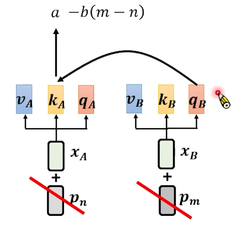
ALiBi's approach: discard Positional Embedding entirely. Compute Attention scores without positional information, then subtract — the relative distance between positions and . This makes Attention smaller for distant tokens. The constant is manually set and can differ per Attention Head.
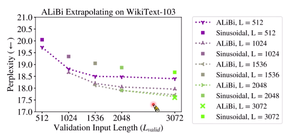
ALiBi outperforms Sinusoidal methods across the board, especially on longer sequences.
T5's Learnable Relative Bias
Reference: https://arxiv.org/abs/1910.10683
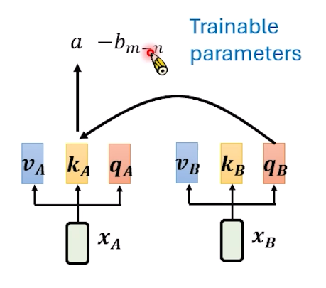
T5 uses a learnable parameter for the bias instead of manually setting it. However, the hand-crafted ALiBi actually outperformed the trained T5 approach.
ALiBi eventually gave way to stronger methods, but its lesson remains: Relative Position matters greatly.
RoPE: Rotary Position Embedding
Reference: https://arxiv.org/abs/2104.09864
RoPE is one of today's most popular methods. Instead of adding a positional embedding, it applies a rotation to and vectors to encode positional information.
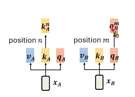
The Attention weight is then:
only depends on the relative position between A and B, directly encoding relative position into the attention computation.
Key advantage: It doesn't affect the Attention computation process itself — only and are modified, and the transformed can be stored in KV Cache.
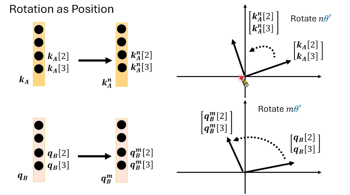
Rotation as Position
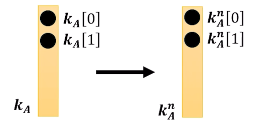
Consider only the first two dimensions of and :
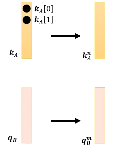
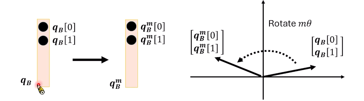
These two dimensions form a vector on a 2D plane.
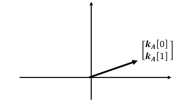
Adding positional information means rotating this vector. To encode position , rotate the first two dimensions of by :
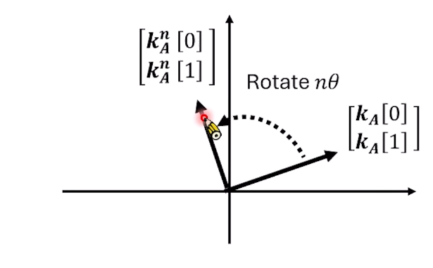
Similarly for , rotate by :
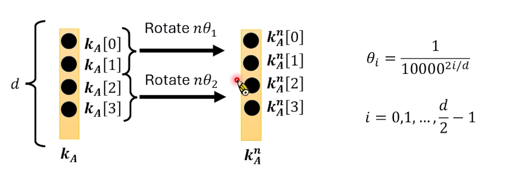
RoPE applies this rotation to every pair of dimensions:
Each pair of dimensions uses a different rotation angle , where:
with .
RoPE's Key Property: Relative Position Invariance
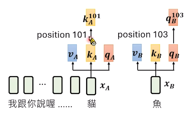
If we move from position to and from to , their relative position stays the same, and the Attention value remains unchanged:
Suppose cat is at position 1 and fish at position 3. We add position 1 to cat's and position 3 to fish's . Fish gets its Query, adds position to get , then computes attention with cat's .
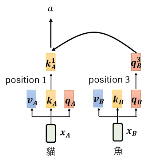
Adding many tokens before cat and fish doesn't affect their Embeddings. If cat is at 101 and fish at 103, the attention value is identical to when cat was at 1 and fish at 3.
Why does RoPE achieve this? Comparing original and with position :
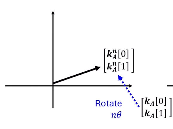
If is moved to position , it is rotated by :
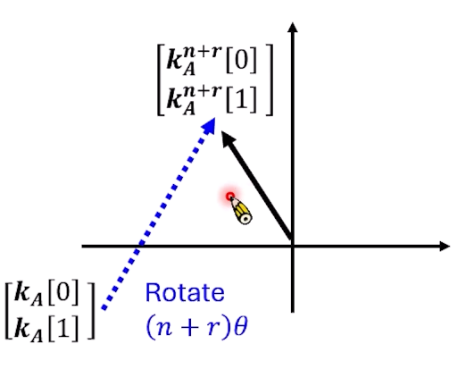
The angle between and is . Same for :
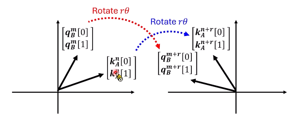
The dot product of and equals that of and , because equal rotation doesn't change the inner product.
RoPE Mathematical Derivation
Let's examine why RoPE only depends on the relative position of and , using the first two dimensions.
Rotating by :
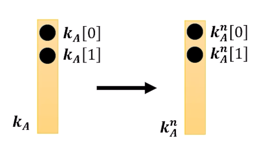
Rotating by :
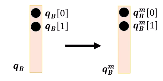
Computing the dot product:
The rotation matrices combine: (transpose) .
Replacing with and with :
Since , the result is identical — confirming relative position invariance.
RoPE Implementation Details
RoPE rotates and separately before computing Attention:
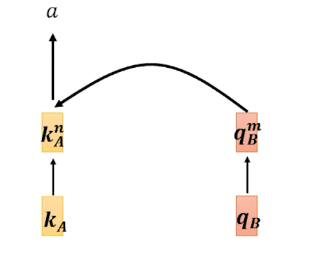
This is equivalent to multiplying by , computing only 's rotation:
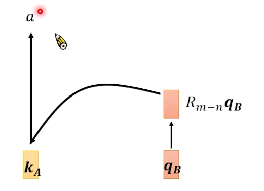
In practice, the first approach is preferred. With the first method, both position-encoded and can be stored in KV Cache. With the second, would need to multiply by different each time. RoPE's compatibility with KV Cache is key to its popularity.
RoPE vs ALiBi: An Important Distinction
Many misunderstand RoPE — thinking like ALiBi, farther and have smaller Attention weights. But RoPE does not guarantee this.
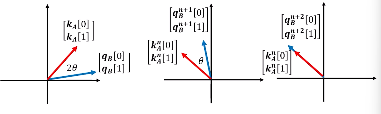
This isn't necessarily a weakness. RoPE can do something ALiBi cannot: skip intermediate tokens to attend directly to earlier ones. In ALiBi, farther tokens always have smaller attention. With RoPE, rotation angles can bring certain positions into alignment regardless of distance.
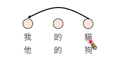
For example, "my cat" and "his dog" — "cat" should attend to "my" and "dog" to "his," not to the middle word "the." RoPE enables this nuanced attention.
If and differ by , but at and at differ by just , and at and at might have the same angle — attention scores can actually increase despite greater distance, allowing the model to skip intermediate tokens.
04 Train Short, Test Long
Reference: https://amaarora.github.io/posts/2025-09-21-rope-context-extension.html
Can we train on short sequences but handle very long sequences during testing without failure?
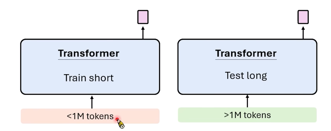
This is crucial for Agents that need to run indefinitely with very large context windows.
During training, we may not have very long corpora. The goal is positional encoding that supports Train Short, Test Long.
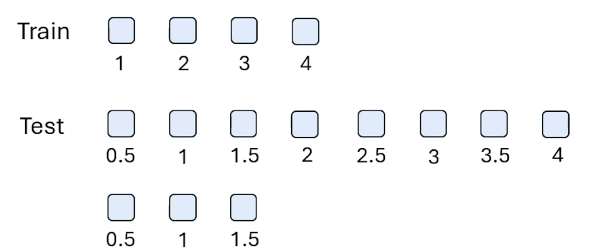
Intuitively, during training we only see tokens with positions .
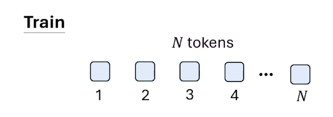
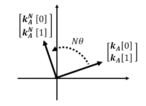
When testing with tokens, can we just assign positions up to ?

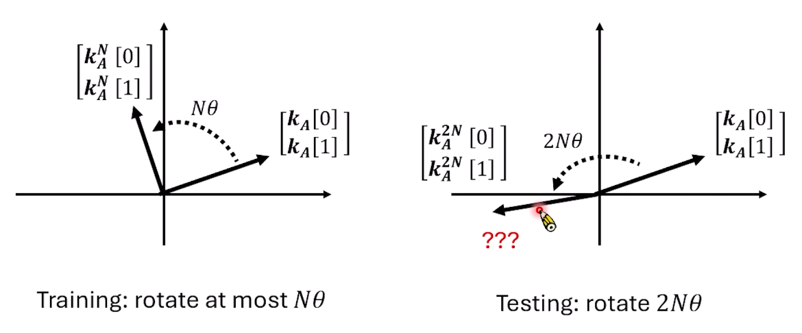
Can RoPE handle this? It seems not.
(From: https://arxiv.org/abs/2108.12409)
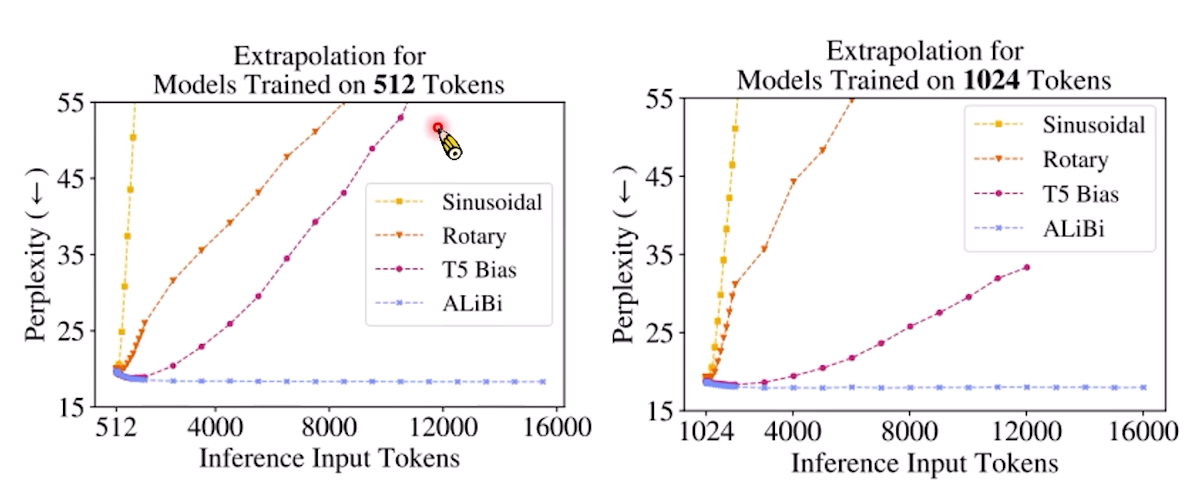
When testing with very long sequences:
- Sinusoidal: fails immediately on longer sequences.
- RoPE: slightly better than Sinusoidal, but also degrades with length.
- ALiBi: the only one that holds up, because it uses hand-crafted rather than learned parameters — proving surprisingly robust.
Why Does RoPE Fail on Long Sequences?
During training, the maximum rotation angle seen is . Testing at presents an angle the model has never seen, and RoPE "freaks out."
Position Interpolation
References:
Solution: don't assign rotation angles beyond .
With tokens, position numbers don't have to be to — they can be to :
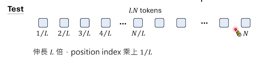
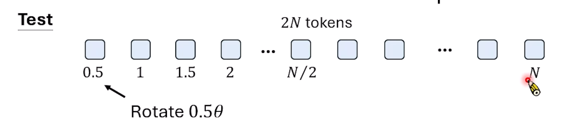
This is Position Interpolation, though it still requires fine-tuning.
Frequency-Based Approach
RoPE processes dimensions in pairs, and Position Interpolation treats all dimensions identically. Frequency-Based Approach asks: can different dimensions be treated differently?
When extending from to , can we multiply by a function that depends on both the extension factor and the dimension?
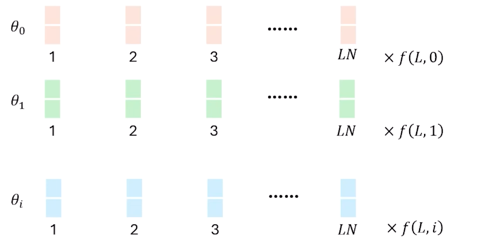
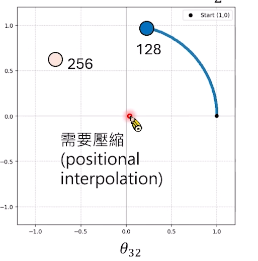
Principle: is high-frequency, larger means lower frequency. High-frequency vectors can stay unchanged; low-frequency vectors need compression.
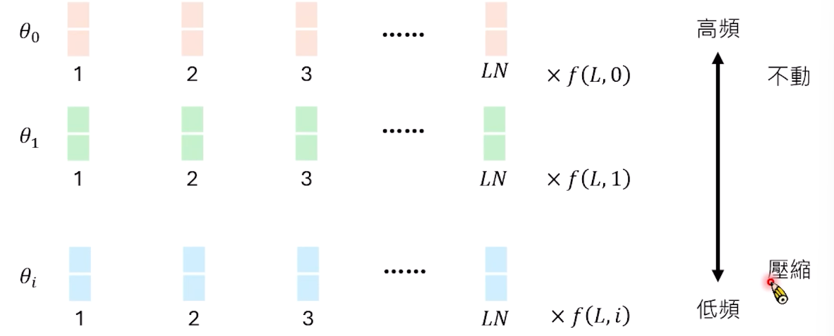
Every two dimensions form a rotating pointer. For the first two dimensions, the pointer rotates very fast. With , may have seen the entire plane many times over, while has barely covered 1/4.
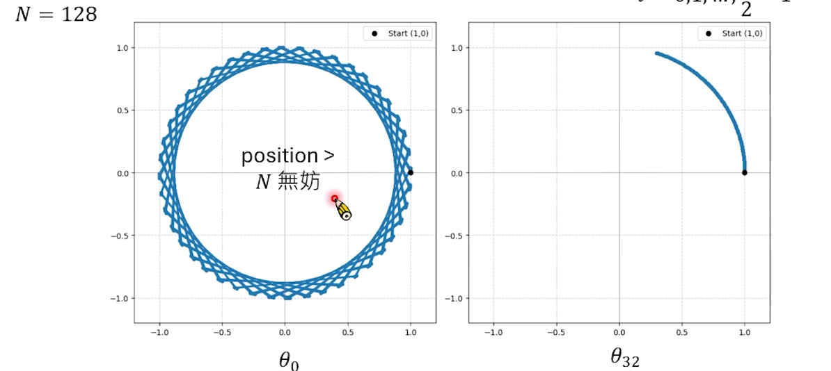
For , positions beyond are fine — it's seen it all. But for , extending to 256 means encountering an unseen rotation angle.
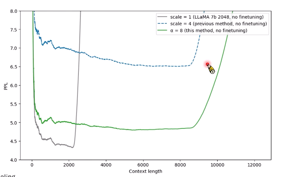
NTK-aware Scaling
Meaning:
- : , no compression at highest frequency.
- : , maximum compression at lowest frequency.
YaRN
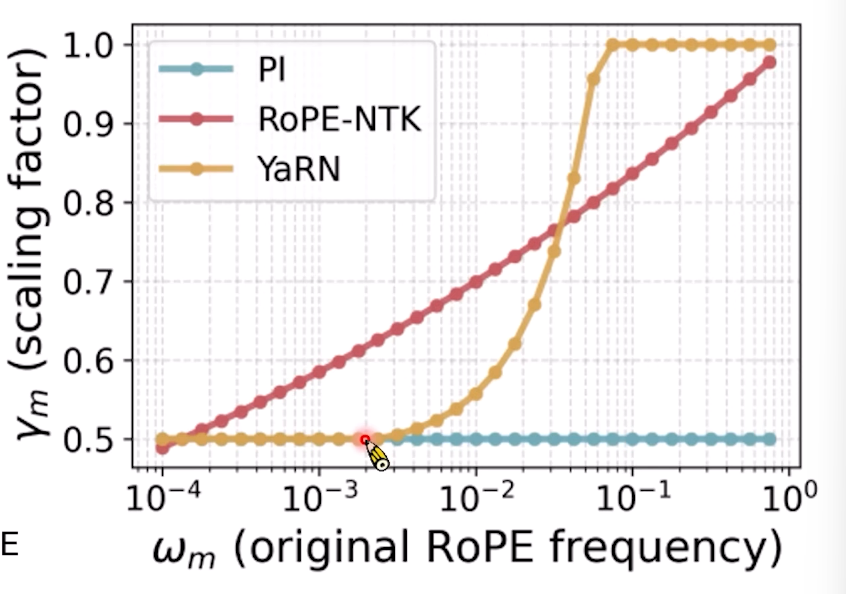
YaRN (Yet another RoPE extensionN method). Reference: https://arxiv.org/abs/2309.00071
Keep some low-frequency scaling unchanged, keep some high-frequency scaling unchanged, only modify the middle frequencies.
Dynamic Scaling
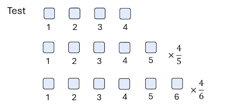
Previous methods handle long sequences, but performance on short sequences may degrade.
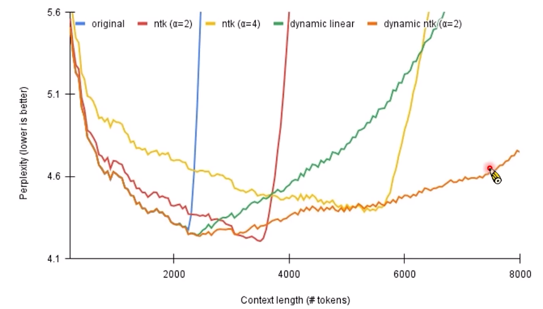
Reference: https://www.reddit.com/r/LocalLLaMA/comments/14mrgpr/dynamically_scaled_rope_further_increases/
Dynamic Scaling: use different treatments for different sequence lengths. For short sequences, don't modify — performance stays good since training saw these lengths.
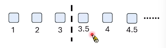
One variant: don't modify positions at the beginning of the sequence, only apply scaling after a certain proportion.
Dynamic Scaling combined with Position Interpolation or NTK outperforms both alone.
Frequency-Based + Dynamic: LongRoPE
Frequency-Based determines the compression function; Dynamic Scaling determines where compression begins. LongRoPE uses Evolutionary Search to find optimal strategies.
Reference: https://arxiv.org/abs/2402.13753
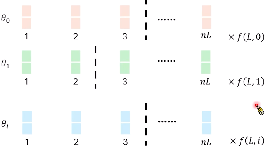
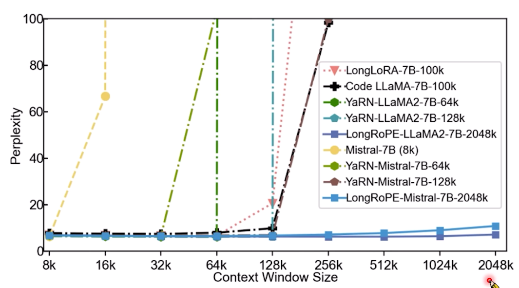
This achieves remarkable results — models handling up to 2048K input length.
05 No Positional Embedding?!
Does Self-Attention Really Have No Positional Information?
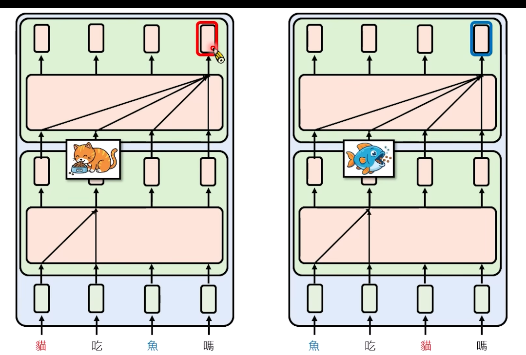
Single-layer Self-Attention has no positional information. But multi-layer Self-Attention is different.
The first layer captures relationships between tokens. The second layer sees these relationships embedded — "cat relates to 'ate'" and "fish relates to 'ate'" produce different representations. So "cat ate fish" and "fish ate cat" yield different final Embeddings even without Positional Embedding.
NoPE: No Positional Embedding
Reference: https://arxiv.org/pdf/2305.19466
Experiments show that No Position Embedding works surprisingly well. On Copy tasks, models with Positional Embedding degraded on long sequences, while NoPE maintained high accuracy.
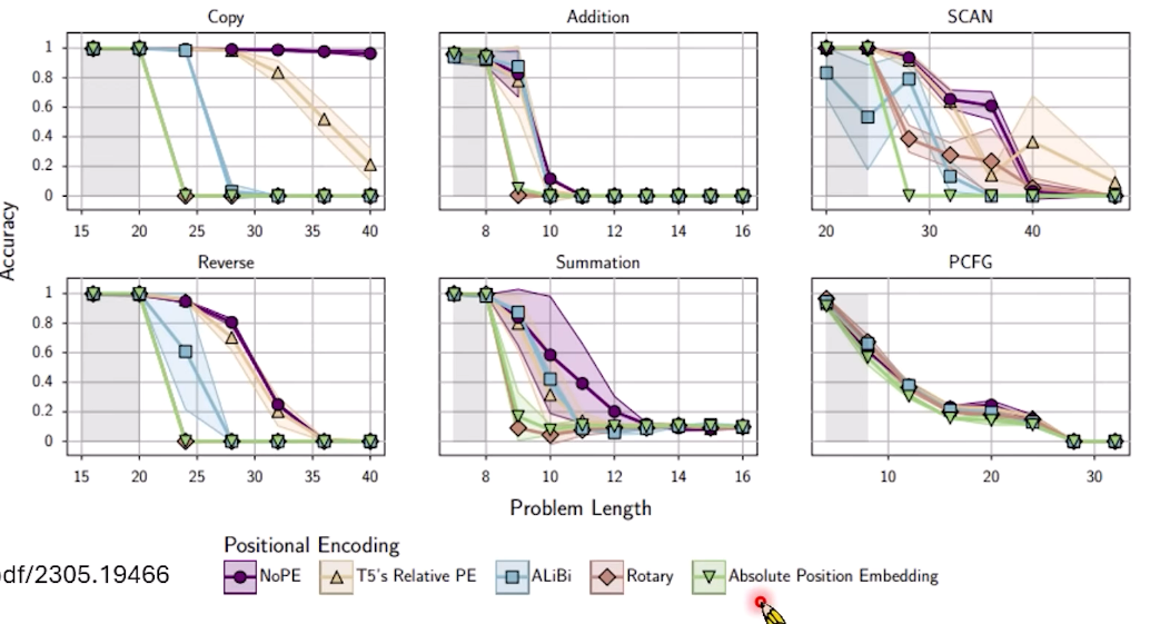
However, comparing RoPE vs NoPE during training — NoPE underperforms RoPE.
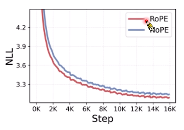
We need Positional Embedding because it helps during training.
DroPE: Dropping Positional Embedding Late in Training
Start training with Positional Embedding, then remove it near the end. Loss spikes briefly but recovers quickly. Training without Position Embedding can match RoPE's loss.
DroPE outperforms RoPE + YaRN on extended contexts. Training at 2K context, then removing positional embedding enables good performance at inference contexts far beyond 2K.
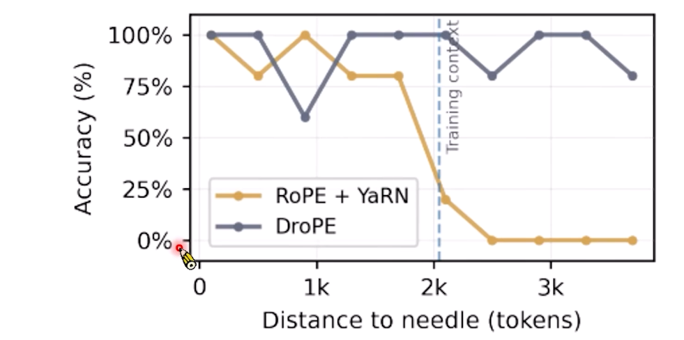
Reference: https://arxiv.org/pdf/2512.12167
References
- Sinusoidal Positional Embedding (Original Transformer)
- ALiBi (Attention with Linear Biases)
- T5 (Text-to-Text Transfer Transformer)
- RoPE (Rotary Position Embedding)
- Train Short Test Long (RoPE Context Extension Survey)
- Position Interpolation
- Position Interpolation (Kaiokendev blog)
- NTK-aware Scaling
- YaRN
- Dynamic Scaling
- LongRoPE
- NoPE
- DroPE
Copyright
Copyright Ownership:
License under: